Basic Concepts
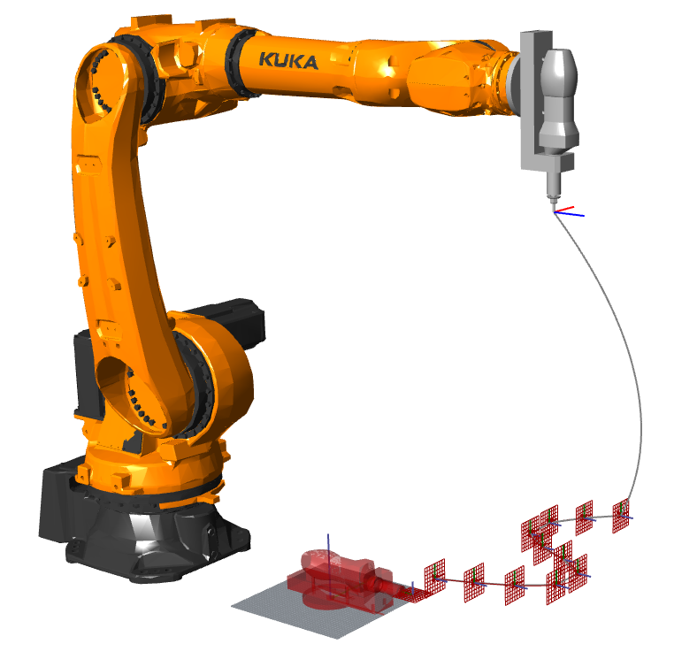
Parametric Robot Control simulates your robot program on the computer and – at the same time – generates the matching program for the robot control. To get from a working simulation to a moving robot, three things have to line up: the program file, the tool, and the base.
From Simulation to Robot Code#
There are non-realtime and realtime drivers. Realtime drivers connect to a robotic system, usually via Ethernet, and control it remotely. That is usually an advanced task. Non-realtime drivers have got less complexity, as they generate a control data file that can then be executed at the robot.
Whenever PRC simulates a task, a non-realtime driver also generates the program in the native language of the robot control – e.g. KRL for KUKA or URScript for Universal Robots. Getting that program is simply a matter of saving it as a file:
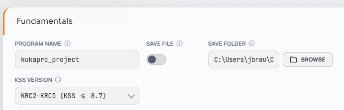
- Open the Robot Settings – either in the browser at
https://localhost:5001, or in Grasshopper by right-clicking the Core component and selecting Show Settings. - Set a Program Name. It is used both as the file name and as the program name inside the code. On some systems like KUKA, special character or empty spaces are not allowed.
- Enable Save File and choose a Save Folder.
- Press Apply Settings.
From then on, every successful simulation writes the current program into the Save Folder – change the toolpath, and the file is updated along with the simulation. The file is saved by the client, i.e. on the computer running Grasshopper, even if the PRC.Server runs on a different machine.
The file format depends on the robot system:
| Robot system | Generated code | File |
|---|---|---|
| KUKA (KSS) | KRL program | .src |
| Universal Robots | PolyScope program / URScript | .urp (PolyScope 5), .urpx (PolyScope X), or .script – set via Selected Polyscope Version |
| ABB | RAPID module | .mod (IRC5) or .modx (OmniCore) – set via IRCVersion |
| NEURA | Python program (NeuraPy) | .py |
Copy the file onto the robot control – typically with a USB stick – and select it on the teach pendant like any manually written program. Some platforms require extra steps. On KUKA robots, the USB drive is by default only visible in a user group like Expert or higher. UR’s Polyscop X requires a robot-specific file - follow the instructions in the help field by creating an empty script with the comment #PRC and then pasting the entire text of the .urpx file in the PRC settings. The placeholder will then be replaced by the PRC-code.
Some drivers skip files entirely: realtime drivers such as the UR Realtime driver send the program to the robot directly over the network.
Tool#
On its own, a robot only knows the position of its flange – the mounting plate at the end of the arm. The tool defines the Tool Center Point (TCP): the working point and orientation of whatever is mounted to that flange, such as the tip of a pen, the nozzle of an extruder, or the rotation axis of a spindle. All Cartesian motions refer to the active TCP – it is the point that follows your toolpath.
If you do not define a tool, PRC uses Tool 0: the flange itself, with no offset.
Defining a tool in Grasshopper:
- Model the tool geometry at the world origin, as if it were mounted on a flange lying flat at the origin.
- Place a plane at the TCP and plug it into a Frame via Plane component. On KUKA robots, the Frame ID is the tool number, e.g.
6for Tool 6. Other system define tools with a string. - Plug the frame and the tool mesh into a Custom Tool component.
- Plug the Custom Tool into the Tool Library input of the Core component.
- Enter the tool number as the Tool ID of every motion group that should use this tool. If you only use a single tool, then PRC will always use the tool connected to the tool library input.
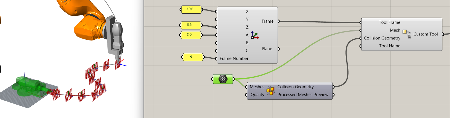
The tool ID is what links the simulation to the physical robot: By default on KUKA robots, the generated code does not contain the tool values themselves, but selects the tool with the same number on the robot control – on a KUKA, for example, TOOL_DATA[6]. Calibrate the tool on the robot (e.g. with the XYZ 4-point method) and use the same values in PRC. If the values in PRC and on the control differ, the real robot will follow a different path than the simulation.
Base#
The base is the coordinate system of your work area: it tells the robot where the workpiece is located. If you do not define a base, PRC uses Base 0, which sits at the robot's own origin.
In PRC, the origin of your CAD environment is the origin of the base: you model the toolpath around the Rhino origin, and the base values describe where that origin is located as seen from the robot. When you change the base values in the settings, the robot in the viewport moves relative to your geometry – the toolpath stays where you modeled it. So if your base is 1000mm in front of the robot, the robot will move 1000mm backwards.
- Open the Robot Settings and go to the Base group.
- Select the Base Number (e.g.
6) and enter its X, Y, Z, A, B, C values. The input fields follow the convention of the respective robot vendor. - Press Apply Settings.
Like the tool number, the base number links simulation and reality: the generated code selects the base with the same number on the control – on a KUKA, for example, BASE_DATA[6]. The proven workflow is to calibrate the base on the robot first, e.g. with the 3-point method, and then enter the measured values in PRC.
For your very first motions, no calibration is needed at all: Axis motions with Tool 0 and Base 0 are the default and will move the robot without any setup.
Simulation Accuracy#
When the tool and base values in PRC match the calibration on the physical robot, and the program starts from a defined axis position, the robot follows the simulated toolpath. The simulation can only be as accurate as the values provided to it. A few differences remain and are good to know abput:
- Rounded corners – Motions are usually approximated: the real robot rounds the transition between two motions (e.g. via
C_DISon a KUKA) to keep moving fluently, while the simulation shows the exact programmed path through every corner. - Cycle time – The simulated duration is an estimate based on the programmed speeds and accelerations. The robot control plans motions with its full dynamic model, and the override slider on the pendant scales all speeds, so real cycle times will differ.
- Start posture – If a program does not start from a clearly defined position, the simulation and the robot may choose different axis configurations to reach the same point. Start every program with an Axis motion – see the Basics section on Getting Started.
- Absolute accuracy – Industrial robots repeat a taught position extremely well (fractions of a millimeter), but their absolute accuracy across the workspace is lower. For precision work, calibrate the tool and base carefully on the physical robot rather than relying on nominal CAD values.
The simulation does not replace care at the machine: always run a new program for the first time at reduced speed (e.g. in KUKA T1 mode), keep your hand on the enabling switch, and keep a safe distance from the robot.